Make a model
Generating: To make a model you need to provide a
DAG statement to make_model. For instance
"X->Y"-
"X -> M -> Y <- X"or -
"Z -> X -> Y <-> X".
# examples of models
xy_model <- make_model("X -> Y")
iv_model <- make_model("Z -> X -> Y <-> X")Graphing: Once you have made a model you can inspect the DAG:
plot(xy_model)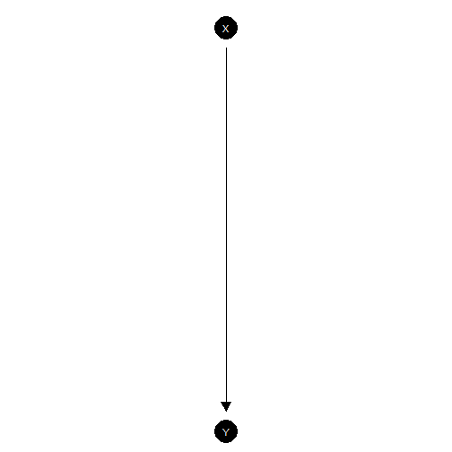
Simple summaries: You can access a simple summary
using summary()
summary(xy_model)
#>
#> Causal statement:
#> X -> Y
#>
#> Nodal types:
#>
#> Nodal types for X:
#> 0  1
#>
#> Nodal types for Y:
#> 00  10  01  11
#>
#> Guide to interpreting nodal types for Y:
#>
#>   index  interpretation
#> 1    *-  Y = * if X = 0
#> 2    -*  Y = * if X = 1
#>
#> Number of nodal types by node:
#> X Y
#> 2 4
#>
#> Number of causal types:  8
#>
#> Note: Model does not contain: posterior_distribution, stan_objects;
#> to include these objects use update_model()
#>
#> Note: To pose causal queries of this model use query_model()
or you can examine model details using inspect().
Inspecting: The model has a set of parameters and a default distribution over these.
xy_model |> inspect("parameters_df")
#>
#> parameters_df
#> Mapping of model parameters to nodal types:
#>
#>   param_names: name of parameter
#>   node:        name of endogeneous node associated
#>                with the parameter
#>   gen:         partial causal ordering of the
#>                parameter's node
#>   param_set:   parameter groupings forming a simplex
#>   given:       if model has confounding gives
#>                conditioning nodal type
#>   param_value: parameter values
#>   priors:      hyperparameters of the prior
#>                Dirichlet distribution
#>
#>   param_names node gen param_set nodal_type given param_value priors
#> 1         X.0    X   1         X          0              0.50      1
#> 2         X.1    X   1         X          1              0.50      1
#> 3        Y.00    Y   2         Y         00              0.25      1
#> 4        Y.10    Y   2         Y         10              0.25      1
#> 5        Y.01    Y   2         Y         01              0.25      1
#> 6 Y.11 Y 2 Y 11 0.25 1Tailoring: These features can be edited using
set_restrictions, set_priors and
set_parameters.
Here is an example of setting a monotonicity restriction (see
?set_restrictions for more):
iv_model <-
  iv_model |> set_restrictions(decreasing('Z', 'X'))
Here is an example of setting priors (see ?set_priors
for more):
iv_model <-
  iv_model |> set_priors(distribution = "jeffreys")
#> Altering all parameters.Simulation: Data can be drawn from a model like this:
| Z | X | Y |
|---|---|---|
| 0 | 1 | 1 |
| 1 | 0 | 0 |
| 1 | 0 | 1 |
| 1 | 1 | 1 |
Update the model
Updating: Update using update_model.
You can pass all rstan arguments to
update_model.
df <-
  data.frame(X = rbinom(100, 1, .5)) |>
  mutate(Y = rbinom(100, 1, .25 + X*.5))

xy_model <-
  xy_model |>
update_model(df, refresh = 0)Inspecting: You can access the posterior distribution on model parameters directly thus:
| X.0 | X.1 | Y.00 | Y.10 | Y.01 | Y.11 |
|---|---|---|---|---|---|
| 0.5237547 | 0.4762453 | 0.1948964 | 0.0523208 | 0.5664182 | 0.1863645 |
| 0.4261285 | 0.5738715 | 0.0597984 | 0.1743038 | 0.6544728 | 0.1114249 |
| 0.5796467 | 0.4203533 | 0.1538045 | 0.1640282 | 0.4844825 | 0.1976849 |
| 0.5133653 | 0.4866347 | 0.0667460 | 0.1497083 | 0.5849814 | 0.1985644 |
| 0.5559260 | 0.4440740 | 0.1106234 | 0.1599240 | 0.6523280 | 0.0771246 |
| 0.5738242 | 0.4261758 | 0.0211059 | 0.3386846 | 0.5650897 | 0.0751198 |
where each row is a draw of parameters.
Query the model
Arbitrary queries
Querying: You ask arbitrary causal queries of the model.
Examples of unconditional queries:
xy_model |>
  query_model("Y[X=1] > Y[X=0]",
              using = c("priors", "posteriors"))
#>
#> Causal queries generated by query_model (all at population level)
#>
#> |label           |using      |  mean|    sd| cred.low| cred.high|
#> |:---------------|:----------|-----:|-----:|--------:|---------:|
#> |Y[X=1] > Y[X=0] |priors     | 0.249| 0.195|    0.009|     0.705|
#> |Y[X=1] > Y[X=0] |posteriors | 0.529| 0.102|    0.313|     0.705|
This query asks the probability that .
Examples of conditional queries:
xy_model |>
  query_model("Y[X=1] > Y[X=0] :|: X == 1 & Y == 1", using = c("priors", "posteriors"))
#>
#> Causal queries generated by query_model (all at population level)
#>
#> |label                                 |using      |  mean|    sd| cred.low| cred.high|
#> |:-------------------------------------|:----------|-----:|-----:|--------:|---------:|
#> |Y[X=1] > Y[X=0] given X == 1 & Y == 1 |priors     | 0.499| 0.283|    0.023|     0.970|
#> |Y[X=1] > Y[X=0] given X == 1 & Y == 1 |posteriors | 0.751| 0.134|    0.479|     0.978|
This query asks the probability that given and ; it is a type of “causes of effects” query. Note that “:|:” is used to separate the main query element from the conditional statement to avoid ambiguity, since “|” is reserved for the “or” operator.
Queries can even be conditional on counterfactual quantities. Here the probability of a positive effect given some effect:
xy_model |>
  query_model("Y[X=1] > Y[X=0] :|: Y[X=1] != Y[X=0]",
              using = c("priors", "posteriors"))
#>
#> Causal queries generated by query_model (all at population level)
#>
#> |label                                  |using      |  mean|   sd| cred.low| cred.high|
#> |:--------------------------------------|:----------|-----:|----:|--------:|---------:|
#> |Y[X=1] > Y[X=0] given Y[X=1] != Y[X=0] |priors     | 0.492| 0.29|    0.027|     0.974|
#> |Y[X=1] > Y[X=0] given Y[X=1] != Y[X=0] |posteriors | 0.809| 0.09|    0.648|     0.980|
Note that we use “:” to separate the base query from the condition rather than “|” to avoid confusion with logical operators.
Output
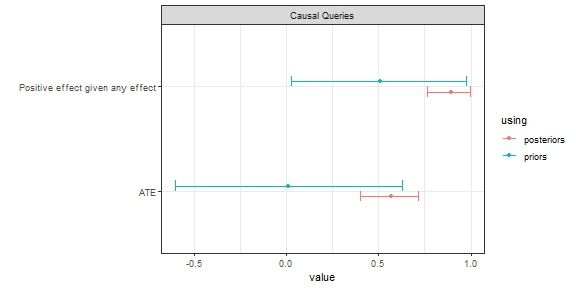
Query output is ready for printing as tables, but can also be plotted, which is especially useful with batch requests:
batch_queries <- xy_model |>
  query_model(queries = list(ATE = "Y[X=1] - Y[X=0]",
                             `Positive effect given any effect` = "Y[X=1] > Y[X=0] :|: Y[X=1] != Y[X=0]"),
              using = c("priors", "posteriors"),
              expand_grid = TRUE)

batch_queries |> kable(digits = 2, caption = "tabular output")| label | query | given | using | case_level | mean | sd | cred.low | cred.high |
|---|---|---|---|---|---|---|---|---|
| ATE | Y[X=1] - Y[X=0] | - | priors | FALSE | 0.00 | 0.31 | -0.64 | 0.63 |
| ATE | Y[X=1] - Y[X=0] | - | posteriors | FALSE | 0.39 | 0.09 | 0.21 | 0.56 |
| Positive effect given any effect | Y[X=1] > Y[X=0] | Y[X=1] != Y[X=0] | priors | FALSE | 0.50 | 0.29 | 0.02 | 0.97 |
| Positive effect given any effect | Y[X=1] > Y[X=0] | Y[X=1] != Y[X=0] | posteriors | FALSE | 0.81 | 0.09 | 0.65 | 0.98 |
batch_queries |> plot()