library(CausalQueries)
library(dplyr)
library(knitr)
library(estimatr)

options(mc.cores = 2)
set.seed(1)
Here we show properties of some canonical causal models, exploring in particular estimates of non-identified queries. The examples include cases where inferences are reliable but also where identification failures result in unreliable posteriors.
Simple experiment
model <- make_model("X -> Y")
model |> plot()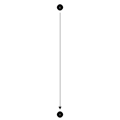
Simple experiment
This model could be justified by a randomized control trial. With a lot of data you can get tight estimates for the effect of on but not for whether a given outcome on is due to . That is the “effects of causes” estimand is identified, but the “causes of effects” estimand is not.
In the illustration below we generate data from a parameterized model
and then try to recover the average treatment effect (ATE) and the
“probability of causation” (POC) for X=1, Y=1 cases. The
ATE has a tight credibility interval. The PoC does not, although it is
still considerably tighter than the prior.
model <- model |>
  set_parameters(nodal_type = c("10", "01"), parameters = c(.1, .6))

data <- model |>
  make_data(n = 5000)

model |>
  update_model(data, refresh = 0, iter = 5000) |>

  query_model(queries =
                list(ATE = "Y[X=1] - Y[X=0]",
                     POC = "Y[X=1] - Y[X=0] :|: X==1 & Y==1"),
              using = c("parameters", "priors", "posteriors")) |>

  plot()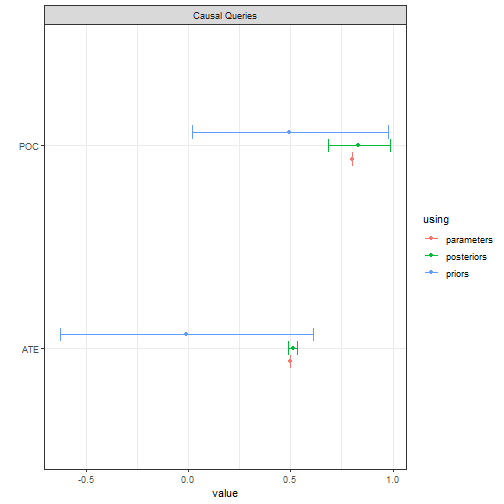
Confounded
model <- make_model("X -> Y; X <-> Y")

model |> plot(x_coord = 0:1, y_coord = 1:0)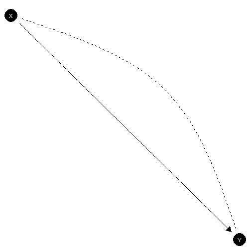
Confounded model
This is the appropriate model if is not randomized and it is possible that unknown factors affect both the assignment of and the outcome .
In the illustration below we use data, drawn from a model in which X is in fact as if randomized (though we do not know this) and there is a true positive treatment effect. We see we have lost identification on the ATE but also our uncertainty about POC is much greater.
model <- model |>
  set_parameters(nodal_type = "01", parameters = .7)

data <- model |>
  make_data(n = 5000)

model |>
  update_model(data, refresh = 0, iter = 5000) |>

  query_model(queries =
                list(ATE = "Y[X=1] - Y[X=0]",
                     POC = "Y[X=1] - Y[X=0] :|: X==1 & Y==1"),
              using = c("parameters", "priors", "posteriors")) |>

  plot()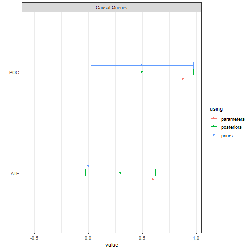
Chain model
model <- make_model("Z -> X -> Y")
model |> plot()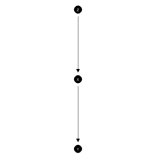
Chain model
This is a chain model. This model is hard to justify from experimentation since randomization of does not guarantee that third features do not influence both and , or that operates on only though .
Even still, it is a good model to illustrate limits of learning about effects by observation of the values of mediators.
Below we imagine that data is produced by a model in which has a 0.8 average effect on and has a 0.8 average effect on . We see that positive evidence on the causal chain (on ) has a modest effect on our belief that caused . Negative evidence has a much stronger effect, albeit with considerable posterior uncertainty.
model <- model |>
  set_parameters(param_names = c("X.10", "X.01", "Y.10", "Y.01"),
                 parameters = c(0.05, .85, .05, .85))

data <- model |>
  make_data(n = 5000)

model |>
  update_model(data, refresh = 0, iter = 5000) |>

  query_model(query = list("Y[Z=1] - Y[Z=0]"),
              given = c("", "Z==1 & Y==1", "Z==1 & Y==1 & X==0", "Z==1 & Y==1 & X==1"),
              using = c("parameters", "posteriors")) |>

  plot()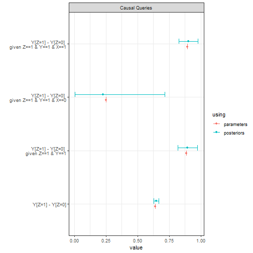
IV model with exclusion restriction
# Model with exclusion restriction and monotonicity
model <- make_model("Z -> X -> Y; X <-> Y") |>
  set_restrictions(decreasing('Z', 'X'))  # monotonicity restriction


# Adding parameters for data generation
model <- model |>
  set_parameters(param_names = c("Y.10_X.01", "Y.01_X.01"),
                 parameters = c(0, .75))     # complier effect

model |> plot(x_coord = c(0,1,0), y_coord = 2:0)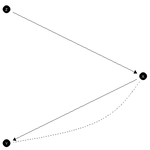
IV model with exclusion restriction satisfied
This is the classic “instrumental variables” model. This model is sometimes justified by randomization of under the assumption that operates on only though (the exclusion restriction). Researchers also often assume that has a monotonic effect on , which we have also imposed here.
Below we draw data from this model, update, and query, focusing our attention on the effects of on for the population and also specifically for units for whom responds positively to , compliers. In addition we ask about the probability of causation, both for units with (PoC) and for compliers with (PoCC). In the model that generated these data an effect is present for compliers only, though researchers do not know (or assume) this.
data <- make_data(model, 4000)

model |>

  update_model(data, refresh = 0, iter = 5000) |>

  query_model(
    query = list(
      ATE = "Y[X=1] - Y[X=0]",
      LATE= "Y[X=1] - Y[X=0] :|: X[Z=1] > X[Z=0]", # ATE for compliers
      PoC = "Y[X=1] - Y[X=0] :|: X==1 & Y==1",    # ATE for units with X=Y-1
      PoCC = "Y[X=1] - Y[X=0] :|: X==1 & Y==1 & (X[Z=1] > X[Z=0])"),    # ATE for units with X=Y-1
    using = c("posteriors", "parameters"),
    cred = 99) |>

  plot()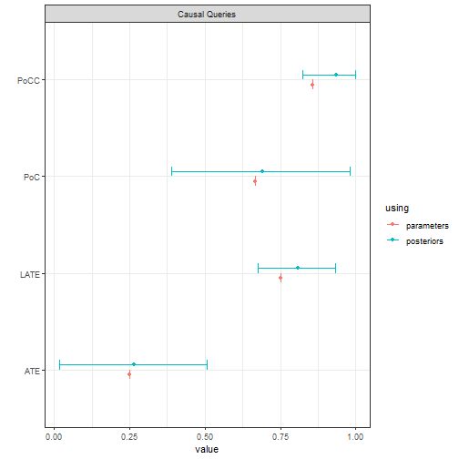
Note the relatively tight posterior for the complier average effect (LATE) and the wide posterior for the average effect and for the probability of causation.
IV model without exclusion restriction
Here is a model in which neither the exclusion restriction or monotonicity holds.
model <- make_model("Z -> X -> Y <- Z; X <-> Y")
model |> plot(x_coord = c(0,1,0), y_coord = 2:0)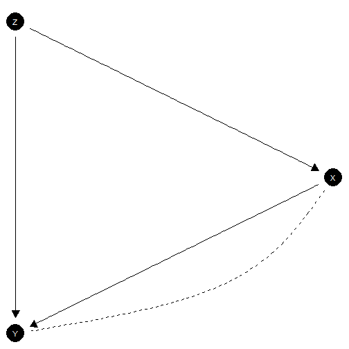
Exclusion restriction not satisfied
Note that for comparability we assume again that the data is the same as before, generated by a model in which the exclusion restriction in fact holds (though researchers do not know this).
model |>

  update_model(data, refresh = 0, iter = 5000) |>

  query_model(
    query = list(
      ATE = "Y[X=1] - Y[X=0]",
      LATE= "Y[X=1] - Y[X=0] :|: X[Z=1] > X[Z=0]", # ATE for compliers
      PoC = "Y[X=1] - Y[X=0] :|: X==1 & Y==1",    # ATE for units with X=Y-1
      PoCC = "Y[X=1] - Y[X=0] :|: X==1 & Y==1 & (X[Z=1] > X[Z=0])"), # ATE for compliers with X=Y-1
    using = c("posteriors"),
    cred = 99
) |>

  plot()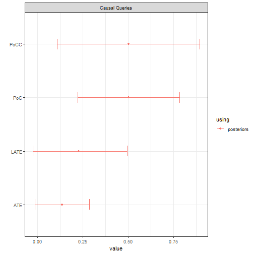
We updated here using a relatively large number of iterations to ensure stable estimates. Note the failure of the two key assumptions are reflected by larger credibility intervals and underestimates for all quantities.
Mediation model with sequential ignorability
model <- make_model("Z -> X -> Y <- Z")

model |> plot(x_coord = c(0,1,0), y_coord = 2:0)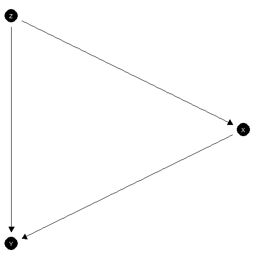
Mediation model with sequential ignorability satisfied
This is a typical mediation type problem where you might want to understand the effects of on that operate directly or that operate via .
We have assumed here that there are no third features that cause both and . This is a strong assumption that is a key part of “sequential ignorability” (see Forastiere et al (2018) for an extensive treatment of the relationship between sequential ignorability and “strong principal ignorability” which we impose here).
Here one might ask queries about different types of direct or indirect effect of on as well as the average effects of on and and of on .
In this example the data is drawn from a world in which the most common type has if and only if both and but in which exerts a negative effect on ; there are both positive direct effects and negative indirect effects.
model <-
  make_model("Z -> X -> Y <- Z") |>
  set_parameters(nodal_type = c("00", "10"), parameters = c(0, .5)) |>
  set_parameters(nodal_type = "0001", parameters = .5)

data <- model |> make_data(n = 2000)

queries <- list(
  `ATE Z -> X` = "X[Z=1] - X[Z=0]",
  `ATE Z -> Y` = "Y[Z=1] - Y[Z=0]",
  `ATE X -> Y` = "Y[X=1] - Y[X=0]",
  `Direct (Z=1)` = "Y[Z = 1, X = X[Z=1]] - Y[Z = 0, X = X[Z=1]]",
  `Direct (Z=0)` = "Y[Z = 1, X = X[Z=0]] - Y[Z = 0, X = X[Z=0]]",
  `Indirect (Z=1)` = "Y[Z = 1, X = X[Z=1]] - Y[Z = 1, X = X[Z=0]]",
  `Indirect (Z=0)` = "Y[Z = 0, X = X[Z=1]] - Y[Z = 0, X = X[Z=0]]"
)

model |>
  update_model(data, refresh = 0, iter = 5000)  |>

  query_model(
    query = queries,
    cred = 99,
    using = c("parameters", "posteriors")) |>

  plot()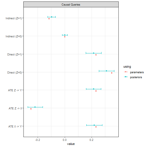
We estimate all quantities very well.
Mediation model without sequential ignorability
We now allow that there may be third features that cause both and . Thus we do not assume “sequential ignorability.” This model might be justified by a random assignment of .
In this example the data is drawn the same way as before which means that in the data generating model the potential outcomes for are independent of those for , though the researcher does not know this. The true (unknown) values of the queries are also the same as before.
model <- make_model("Z -> X -> Y <- Z; X <-> Y")  |>
  set_parameters(nodal_type = c("00", "10"), parameters = c(0, .5)) |>
  set_parameters(nodal_type = "0001", parameters = .5)

model |> plot(x_coord = c(0,1,0), y_coord = 2:0)
  model |>

  update_model(data, iter = 5000) |>

  query_model(
    query = queries,
    cred = 99,
    using = c("parameters", "posteriors")
    ) |>

  plot()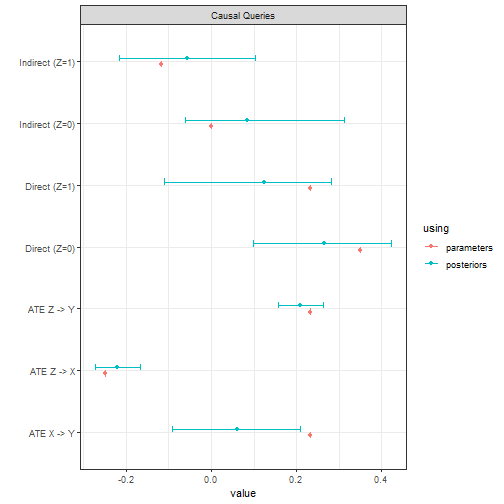
We see we do not do nearly so well. To ensure stable estimates we ran a large number of iterations. For the non-identified quantities our credibility intervals are not tight (which is as it should be!) and in one case the true value lies outside of them (which is not as it should be). This highlights the extreme difficulty of this problem. Nevertheless the gains relative to the priors are considerable.
The napkin model
model <- make_model("W->Z->X->Y; W <-> X; W <-> Y")
plot(model)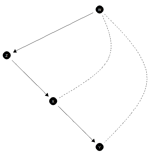
The “napkin” model (see Pearl’s Book of Why) involves two types of confounding. We will paramaterize a version in which (a) the average causal effect of on is negative, arising in cases when (b) there is positive confounding arising from the fact that is liable to be 1 regardless of when and ) is liable to be 1 regardless of when .
model <- model |>
  set_parameters(param_name = "Y.10_W.0", parameters = .6) |>
  set_parameters(param_name = "Y.11_W.1", parameters = .9) |>
  set_parameters(param_name = "X.11_W.1", parameters = .9)
Naive regression performs very badly here.
data <- make_data(model, n = 5000, using = "parameters")

 estimatr::lm_robust(Y ~ X, data = data)  |>
   tidy() |>
kable(digits = 2)| term | estimate | std.error | statistic | p.value | conf.low | conf.high | df | outcome |
|---|---|---|---|---|---|---|---|---|
| (Intercept) | 0.75 | 0.01 | 66.39 | 0 | 0.73 | 0.78 | 4998 | Y |
| X | -0.05 | 0.01 | -3.63 | 0 | -0.08 | -0.02 | 4998 | Y |
In contrast, the updated causal model yields good estimates for the ATE, though again we have somewhat more uncertainty for the probability of causation.
model |>
  update_model(data, refresh = 0, iter = 6000) |>
  query_model(
    list(
      ATE = "Y[X=1] - Y[X=0]",
      PoC = "Y[X=1] - Y[X=0] :|: X==1 & Y==1"),
    using = c("posteriors", "priors", "parameters")) |>
  plot()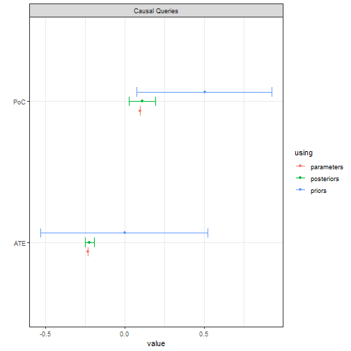
M-bias
In the below model, also studied in Pearl (Causality), the effect of on is identified without controlling for . Controlling for , however, introduces a backdoor path between and which can introduce bias in naive estimation.
Strikingly might be prior to but it can still introduce bias. Here is the model
model <- make_model("Z <- U1 -> Y; Z <- U2 -> X; X -> Y")Here is a parameterization in which there is no true effect of on yet a strong negative correlation between and once you control for .
model <- model |>
  set_parameters(param_name = "Y.0101", parameters = .8) |>
  set_parameters(param_name = "Z.0001", parameters = .8) |>
  set_parameters(param_name = "X.01", parameters = .8)


plot(model)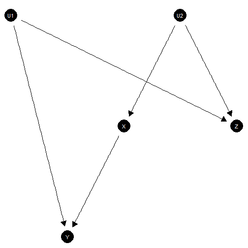
With this model, naive regression results perform poorly when you control for .
data <- model |> make_data(n = 1000)


list(
  `no controls` = estimatr::lm_robust(Y ~ X, data = data),
  `with controls` = estimatr::lm_robust(Y ~ X + Z, data = data)
) |>
   lapply(tidy) |> bind_rows(.id = "Model") |>   filter(term =="X") |>
kable(digits = 2, caption = "Estimation with and without controls")| Model | term | estimate | std.error | statistic | p.value | conf.low | conf.high | df | outcome |
|---|---|---|---|---|---|---|---|---|---|
| no controls | X | 0.04 | 0.03 | 1.32 | 0.19 | -0.02 | 0.10 | 998 | Y |
| with controls | X | -0.11 | 0.03 | -3.48 | 0.00 | -0.18 | -0.05 | 997 | Y |
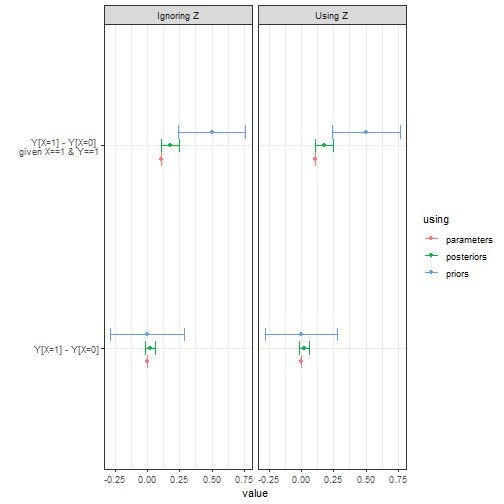
Taking account of does not harm (and could help) in the Bayesian setting.
list(
  `Using Z` = model |> update_model(data, iter = 5000),
  `Ignoring Z` = model |> update_model(data |> dplyr::select(-Z), iter = 5000))|>

  query_model(
    list(
      "Y[X=1] - Y[X=0]",
      "Y[X=1] - Y[X=0] :|: X==1 & Y==1"),
    using = c("parameters", "priors",  "posteriors")) |>

  plot()